Robot Calibration (Laser Tracker)
Introduction
Industrial robot arms are highly repeatable but not accurate, therefore the accuracy of an industrial robot can be improved through robot calibration. The nominal accuracy of a robot depends on the robot brand and model. With RoboDK and the robot calibration option you can improve robot accuracy by a factor of 2 to 10.
With RoboDK you can calibrate 6-axis robot arms and you can obtain accuracies up to 0.050 mm for small robots and 0.150 mm for medium sized robots. The accuracy you can obtain after calibration highly depends on the robot model and your setup. With RoboDK you can’t calibrate 5-axis or 7-axis robot arms.
A measurement system is required to calibrate a robot. RoboDK can be used to calibrate the robots as well as to generate accurate robot programs (this includes filtering the programs and using RoboDK’s offline programming engine). RoboDK can also be used to test the accuracy of the robot before and after calibration through ballbar testing or robot milling.
Robot calibration can remarkably improve the accuracy of robots programmed offline, also known as Off-Line Programming (OLP). A calibrated robot has a higher absolute as well as relative positioning accuracy than an uncalibrated one.
Requirements
The following hardware and software components are required to properly perform robot calibration with RoboDK.
1.One or more robot arms (6-axis robot arm).
2.A measurement system: any laser tracker such as Leica, API or Faro and/or optical CMM such as the C-Track stereocamera from Creaform should work. The corresponding software to communicate with the measurement system should also be installed. For example, Leica trackers don’t need additional software to be installed, on the other hand, the C-Track system requires VxElements with the VxTrack and VxModel options installed.
3.RoboDK software must be installed and an appropriate license for robot calibration testing is required. For network licenses, an internet connection is required to check the license. To install or update RoboDK for robot calibration:
a.Download RoboDK from the website: https://robodk.com/download.
b.Set up the driver for the measurement system (not required for latest Leica trackers)
Unzip and copy the subfolder in:
C:/RoboDK/api/
API Laser tracker: https://robodk.com/downloads/private/API.zip (OTII and Radian trackers).
Faro Laser Tracker: https://robodk.com/downloads/private/Faro.zip(all Faro Trackers).
Leica Laser Tracker: https://robodk.com/downloads/private/Leica.zip (all Leica Trackers).
4.When using a laser tracker, one or more targets should be attached to the robot tool. Important: Make sure to avoid placing the target near axis 6 during the tool setup. Otherwise, it is not possible to properly identify the location of the robot flange ([X, Y] coordinates of the TCP should not be [0,0].
Offline Setup
It is recommended to create a virtual environment of the robot setup in RoboDK (offline setup) before starting to take measurements. This section explains how to prepare the RoboDK station offline. This can be done before having the robot and the tracker, only using a computer with RoboDK installed.
RoboDK calibration project examples can be downloaded from the library of sample stations.
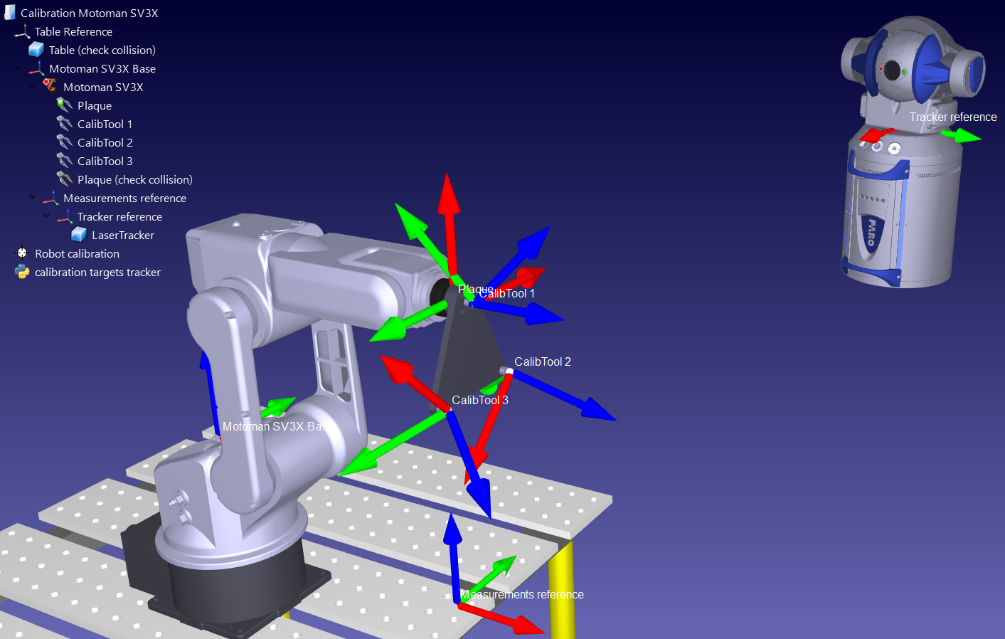
Skip this section if you already have an offline cell. The reference frames and tool frames can be estimated approximately. A sample station is shown in the following picture.
RoboDK station
A RoboDK station is where the virtual environment station and calibration information is stored. The station is saved as an RDK file. Follow the next steps to create a robot station for robot calibration from scratch (video preview: https://youtu.be/Nkb9uDamFb4):
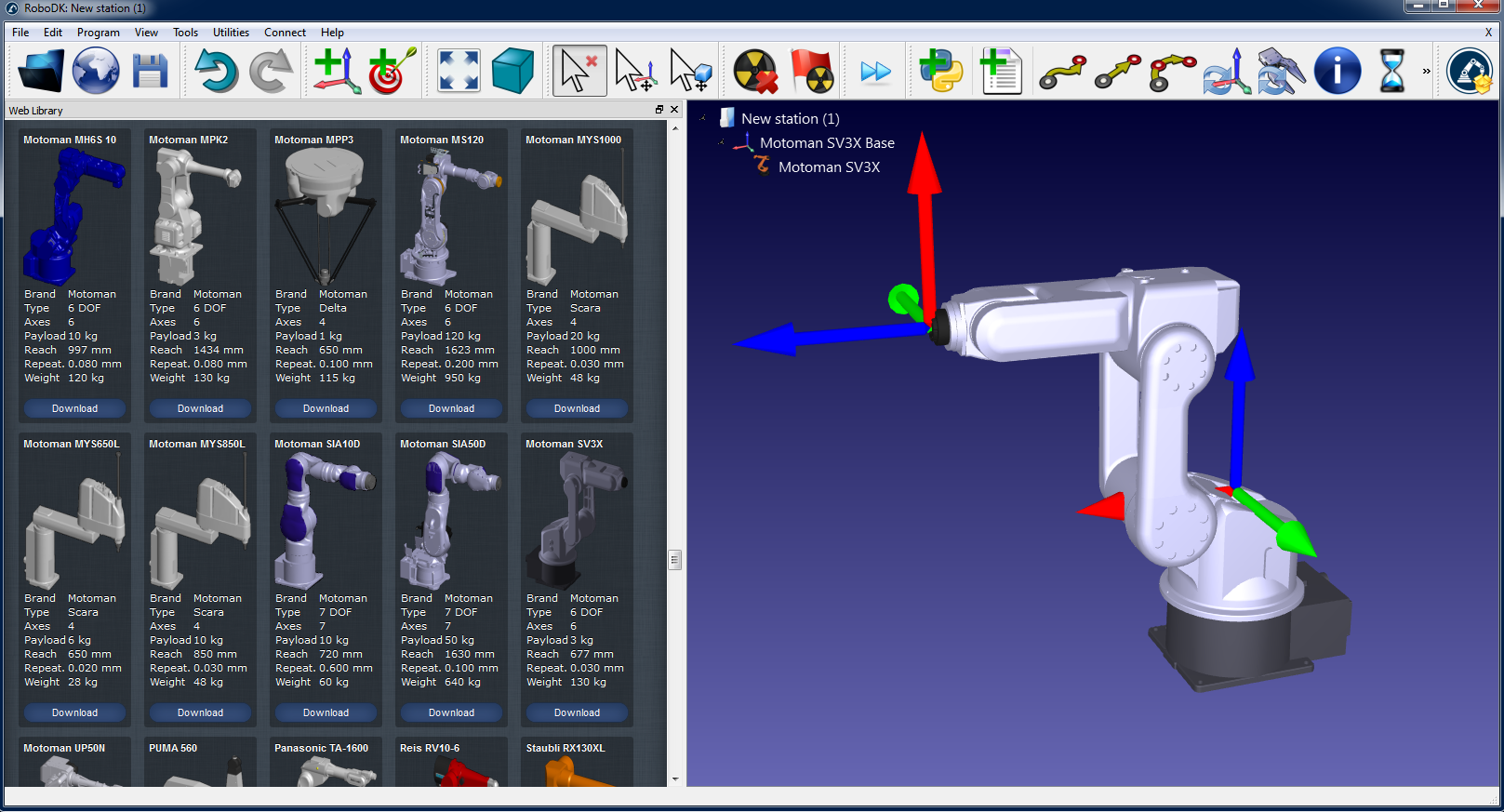
1.Select the robot:
a.Select File➔Open Robot library. The online library will open in your browser.
b.Use the filters to find your robot by name, brand, payload, ...
c.Select Open and the robot should automatically appear in your open RoboDK project.
d.Alternatively, you can download the robot files (.robot file) from http://robodk.com/library and open them with RoboDK.
2.Prepare your project for robot calibration:
a.Add reference frames by selecting Program➔Add Reference Frame.
i.One “Measurements reference” frame must be added with respect to the robot base frame.
ii.One “Tracker reference” must be added with respect to the “Measurements reference” that you just added.
iii.One additional “Tool reference” can be optionally added with respect to the “Measurements reference” frame to visualize the position of the tool seen by the tracker.
b.Add the tool object (STL, IGES and STEP files are supported formats) and drag and drop it to the robot (within the item tree), this will automatically convert the object into a tool. More information available here.
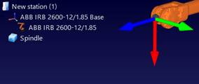
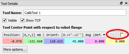
Optional: Select Program➔Add Tool (TCP) to add any TCP’s that you want to visualize in the station (to check for collisions or other). To set an approximate value of the TCP:
i.Double click the new tool.
ii.Set an approximate TCP value. You can copy/paste the 6 values at once using the two buttons at the right.
iii.It is recommended to rename the TCPs used for calibration with the name “CalibTool id”, where id is the calibration target number.
c.Add other 3D CAD files (STL, IGES, STEP, SLD, ...) to model the virtual station using the menu File➔Open… Alternatively, drag and drop files to RoboDK’s main window.
3.Add the calibration module in the station:
a.Select the menu Utilities➔Calibrate Robot.
b.Select Points (3 DOF). You can optionally select Poses (6 DOF) if you have a laser tracker that can take pose measurements and is compatible with RoboDK (such as the Leica T-Mac laser tracker).
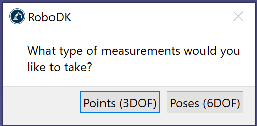
Then, the following window will appear.
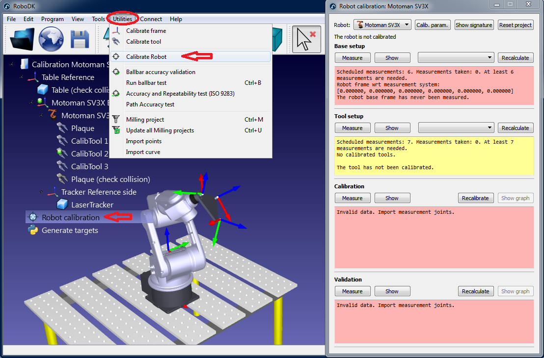
This window can be closed for now. You can open it anytime by double clicking the Robot calibration station item.
4.Save the station.
a.Select File➔Save Station.
b.Select a folder and choose a file name.
c.Select save. A new RDK file will be generated (RoboDK station file).
You can recover the station modifications anytime by opening the RDK file (double click the file).
Summarizing, it is important to double check the following points:
1.The calibration tool (SMR target) should be called “CalibTool 1”. It is strongly recommended to start the calibration with only 1 tool/target. If you have more calibration targets you should increase the index accordingly. For example, if you have 3 calibration tools/SMRs you should name them “CalibTool 1”, “CalibTool 2” and “CalibTool 3”.
2.The Measurements reference frame directly depends on the robot base.
For now, you can use an estimate of this reference frame.
3.The Tracker reference should be directly attached to the Measurements reference. The tracker reference must be an approximate position of the laser tracker with respect to the measurements reference. The Base setup will properly adjust the tracker location.
4.The Robot calibration project is present in the station and all the measurements that you are planning to take are free of collision and visible by the laser tracker (select show for each group of measurements).
5.If you want to automatically check for collisions, you should use the name tag “collision” in every object that you want to use to check collisions. It is recommended to use a tool around 25% bigger than the calibrated tool for collision checking to safely avoid collisions.
Generate calibration targets
There are four sets of measurements that are required to successfully accomplish robot calibration:
1.Base setup: six measurements (or more) moving axis 1 and 2 are required to place the calibration reference with respect to the robot. Select Show in the calibration settings window and the robot will move along the sequence.
2.Tool setup: seven or more measurements are required to calibrate the tool flange and the tool targets (moving axis 5 and 6). Select Show and the robot will move along the sequence.
3.Calibration measurements: 60 measurements or more are required to calibrate the robot. These measurements can be randomly placed in the robot workspace and free of collision with the surrounding objects.
4.Validation measurements (optional): schedule as many measurements as desired to validate the accuracy of the robot. These measurements are used only to validate the accuracy of the robot and not to calibrate the robot.
The first two sets of measurements are automatically generated by RoboDK. Select Show and the robot will follow the sequence (as shown in the following images). If the sequence needs to be changed, select Measure and export the calibration measurements as a CSV file by selecting Export data. This file can be edited using an Excel sheet and re-imported by clicking Import data.
The last two sets of measurements (calibration and validation) can be generated using the macro script called Create measurements. This script is automatically added to the station when you start the robot calibration project. Double click the macro to execute it. This is a Python program that guides the user to define the following settings:
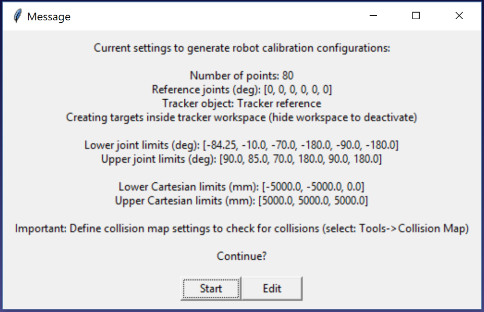
●Number of measurements: The number of measurements to generate. By default, 80 measurements are used because a minimum of 60 measurements is required for robot calibration.
●Reference position: The reference position must be a position of the robot where the tool is facing the tracker with visible targets.
●Joint limits: The lower and upper joint limits must be provided.
●Cartesian limits: You can provide Cartesian limits (X,Y,Z values) with respect to the robot reference frame.
The script automatically generates measurements where the tool is facing the tracker as well as respecting the joint and Cartesian constraints. A rotation of +/-180 deg around the tool is permitted around the direction that faces the tracker at the reference position. Furthermore, the sequence of joint movements is free of collision and inside the measurement workspace (if the workspace is set to be visible). The following image shows the summary that is presented to the user before the automatic sequence starts. It may take up to 5 minutes for the sequence to finish.

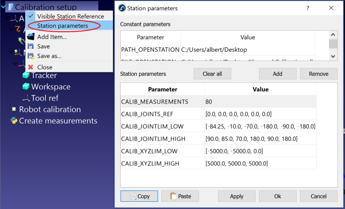
If desired, you can modify the script by right clicking the Create measurements script and selecting Edit script, then, modify additional parameters of the algorithm. The script automatically saves the user input as station parameters. You can view, edit or delete these settings by right clicking the station and selecting Station parameters, as shown in the next image.
A new message will pop up once the algorithm finishes. You can select “Calibration” to use the 60 measurements for robot calibration. You can re-execute the same script to generate another set of measurements for validation. This step is optional, but 80 measurements are recommended for validation purposes.
Finally, it is also possible to import configurations that have been selected manually by selecting Import data (inside the Measure menu). You can import a CSV or a TXT file as an Nx6 array of values, where N is the number of configurations.
Robot calibration setup
You should make sure you have a proper setup to obtain the best accuracy after calibration.
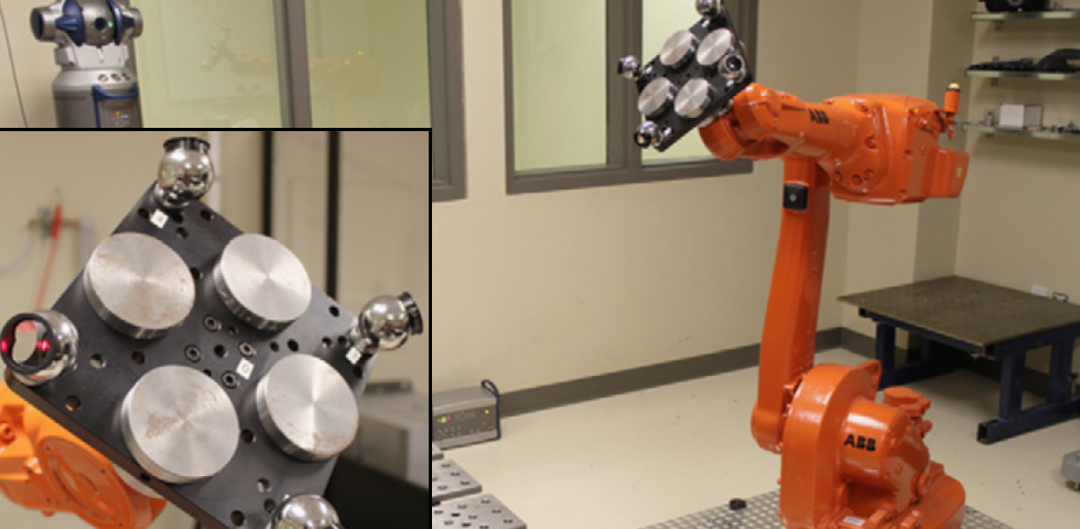
You should first connect the laser tracker. You can optionally connect your robot to the computer to fully automate the procedure of taking measurements.
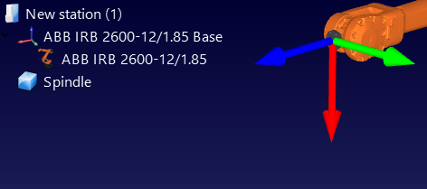
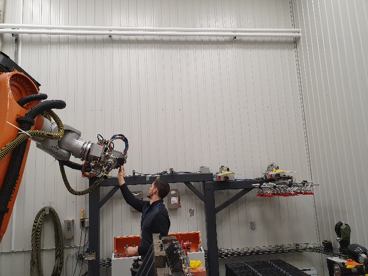
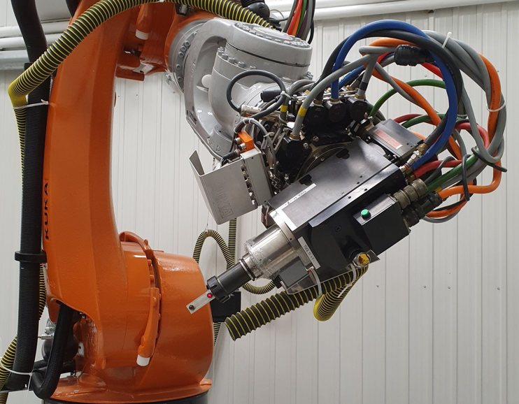
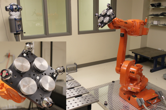
Also, make sure to attach at least one SMR target as shown in the following images. One SMR should be enough to have accurate results. We recommend you place the SMR target close to the TCP of interest. For example, if you are going to use your robot for robot machining, you could try placing one SMR on the cutting axis of your spindle.
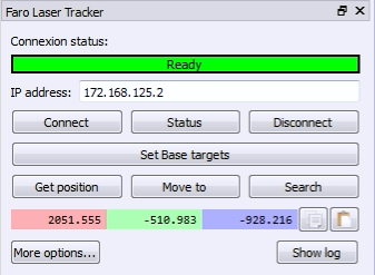
Connect to the tracker
The IP of the laser tracker is needed to properly set the communication with RoboDK. Follow these steps to verify the communication with the laser tracker:
a.Select the menu « Connect➔Connect laser tracker ». A new window should open.
b.Set the IP of the laser tracker.
c.Click the “Connect” button.
If the connection is successful you should see a green message showing “Ready”. The window can be closed and the connection will remain active.
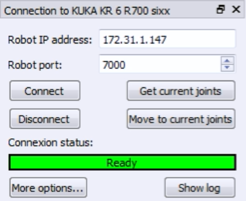
Connect to the robot
The IP of the robot (or the COM port number for RS232 connections) is needed to properly set the communication with RoboDK. Follow these steps to verify the communication with the robot:
1.Select Connect➔Connect robot. A new window will appear.
2.Set the IP and port of the robot (or the COM port if the connection is through RS232).
3.Click the Connect button.
4.Refer to the appendix if any problems arise.
If the connection is successful, you should see a green message displaying Ready. The position of the virtual robot should exactly match the position of the real robot if you select Get Position. Alternatively, select Move Joints to move the robot to the current position in the simulator. You can close this side window for now and the connection will remain active.

Measuring the reference targets
You can use a calibration reference frame if you are planning to move the laser tracker during the calibration or you would like to recover mastering for axis 1.
The calibration reference should be attached to the robot base, this will be helpful if you want to move the tracker during calibration or compare two robot calibrations. The calibration reference frame must be defined by 3 tangible points or SMRs.
You can skip this step if you are not going to move the tracker with respect to the robot or you don’t need to recover the home position for axis 1. In this case, the reference of the laser tracker will be used.
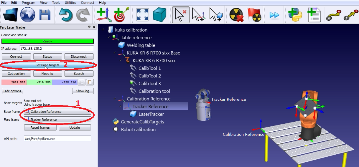
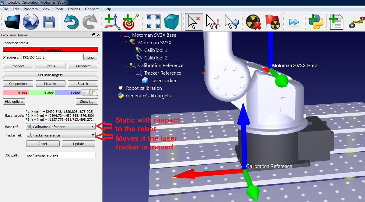
You should follow these steps every time the laser tracker is moved:
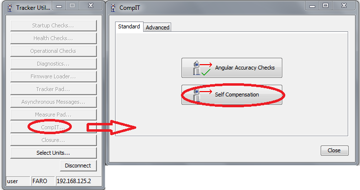
1.Select Connect➔Connect Faro Laser Tracker. Or the corresponding tracker you have.
2.Set the IP of the laser tracker and select connect (if laser tracker is not connected).
3.Set the calibration reference and the tracker reference as shown in the image. The calibration reference is also known as “Measurements reference”.
4.Select Set Base targets.
RoboDK will guide the user with the menus shown in the next image. The position of the laser tracker will be updated automatically with respect to the calibration reference when the procedure is completed.
Robot calibration
Robot calibration is divided in 4 steps. Each step requires taking a set of measurements. These four steps must be followed in order:
1.Base reference measurements (3 minutes).
2.Tool reference measurements (3 minutes).
3.Calibration measurements (7 minutes, 60 measurements).
4.Validation measurements (7 minutes, 60 measurements).
The following video shows how to perform this calibration in 20 minutes: https://www.robodk.com/robot-calibration#tab-lt. The validation measurements (step 4) are not mandatory to calibrate the robot, however they provide an objective point of view of the accuracy results. It is also possible to see the impact of calibrating the robot in one area and validating it in a different area.
Select the button Measure for each of the four sets of measurements. This will open a new window that allows taking new measurements as well as import and export existing measurements in a text file (csv or txt format).
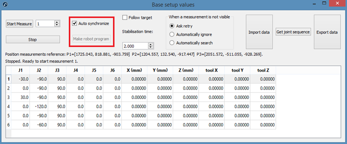
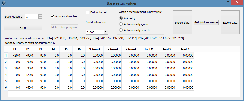
By default, the robot and measurement system are automatically synchronized through the connected robot. If a robot driver is not available, you can still perform robot calibration by generating a robot program which will prompt the user on the teach pendant for manual synchronization.
1.Uncheck Auto synchronize.
2.Click on the Make robot program button.
3.Use the proper post processor to generate the robot program.
Measuring the base
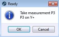
These measurements can be performed anywhere in the tool flange if you measure the same target for all the 6 measurements. To start the measurements, select Measure in the Base setup section. The following window will open. Then, select Start Measure and the robot will move sequentially through the scheduled measurements.
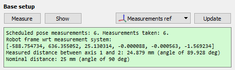
Close the window when the measurements are completed, and the Measurements reference frame will be updated with respect to the robot base frame. If you didn’t select any reference frame, you can add a reference (select Program➔Add Reference Frame) and place it under the robot base reference (Drag & Drop in the item tree).
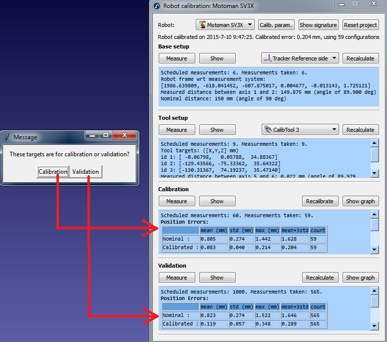
The summary will show the position and orientation or the robot reference frame with respect to the calibration reference frame ([x,y,z,w,p,r] format in mm and radians)
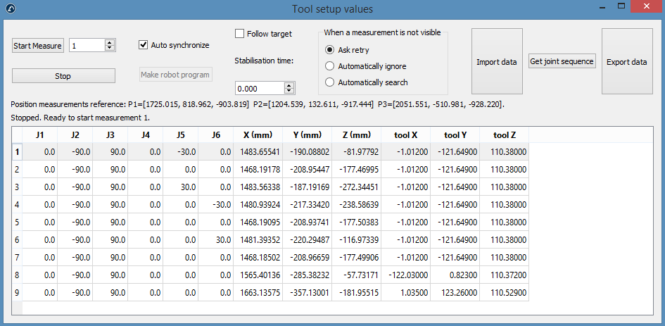
Measuring the tool
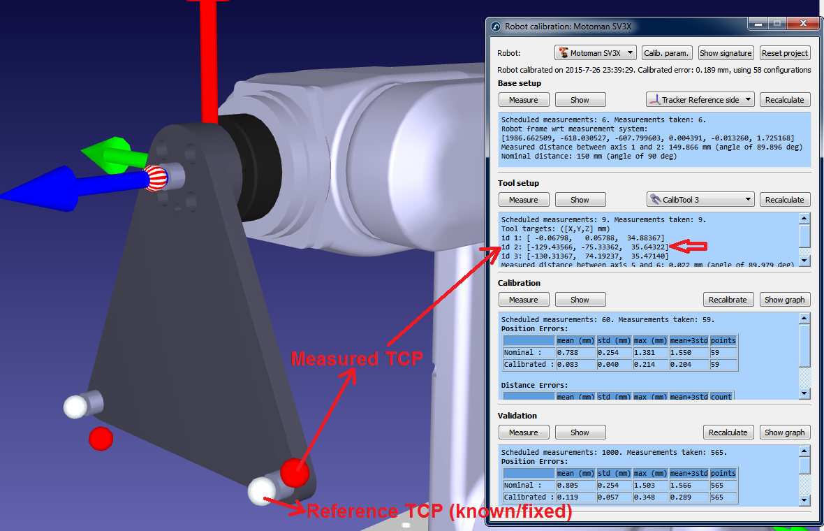
Measurements 1-6 can be performed anywhere in the tool flange as long as you measure the same target for the 6 measurements. After that, every TCP that you want to measure will add one measurement for the same TCP, in this case, you have 3 TCPs so 6+3=9 measurements in total. You can double click a measurement to continue measuring from that position.
Like the previous section: select Measure in the Tool setup section. The following window will open. Select Start Measure and the robot will move sequentially through the planned measurements. Double click a measurement to continue measuring from that position.
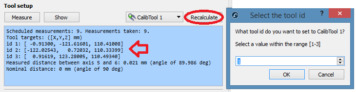
The summary will show the calibrated TCPs when the procedure is completed. The definition of the TCP (in the following image “CalibTool 1”) will be updated automatically. If you didn’t select any TCP, you can add a new one (select “Program➔Add empty Tool”) and select “Recalculate”. A new window will appear, and you must select the “id” of the tool depending on the order that you took the measurements. You can repeat the same procedure to update as many TCPs as you need (in this case 3 TCPs). The id of the tool will be automatically detected if the name of the tool ends with a number.
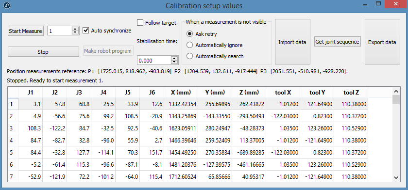
Calibration
Select Measure in the Calibration section to open the robot calibration measurements window. Then, select Start Measure and the robot will move sequentially through the planned measurements. Double click a measurement to continue measuring from that position.
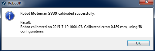
Close the window when the measurements are completed. The robot will be calibrated automatically and it will display the following message if there are no issues.
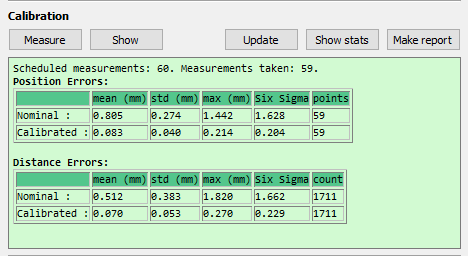
Finally, the green screen will display some statistics regarding the calibration measurements and how much the accuracy is improved for those measurements.
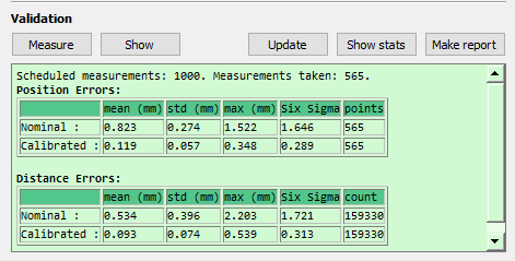
Validation
You shouldn’t validate the accuracy of the robot using the same measurements that you used to calibrate the robot, therefore, it is recommended to take additional measurements to validate the accuracy (having a more objective point of view of the accuracy results).
The same calibration procedure must be followed to take the validation measurements. The summary will display the validation statistics. See the following Results Section for more information.
Results
Once the calibration is completed you can analyze the accuracy improvement by reading the statistics provided by RoboDK. To display these statistics, open the robot calibration window (double click the icon Robot Calibration). The summary window in the validation section will display the errors before calibration (nominal kinematics) and after calibration (calibrated kinematics). Two tables are provided, one shows statistics concerning position errors and the other one shows distance errors:
●Position errors: The position error is the accuracy with which the robot can reach a point with respect to a reference frame.
●Distance errors: The distance error is obtained by measuring the distance error of pairs of points. The distance between two points seen by the robot (obtained using the calibrated kinematics) is compared with the distance seen by the measurement system (physically measured). All combinations pairs are taken into account. If you took 315 measurements you will have 315x314/2= 49455 distance error values.
The statistics provided are the mean error, the standard deviation (std) and the maximum error. It is also provided the mean plus three times the standard deviation, which corresponds to the expected error for 99.98% of all the measurements (if you take into account that errors follow a normal distribution).
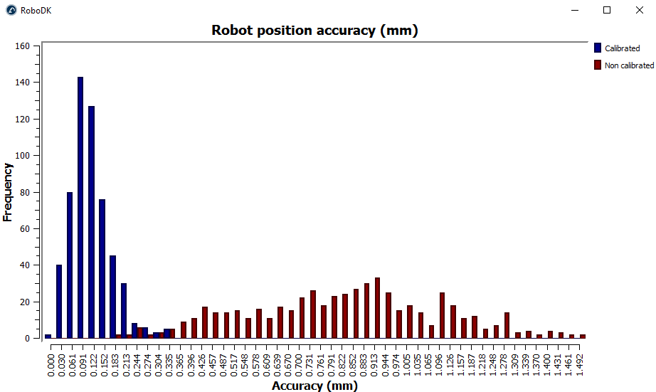
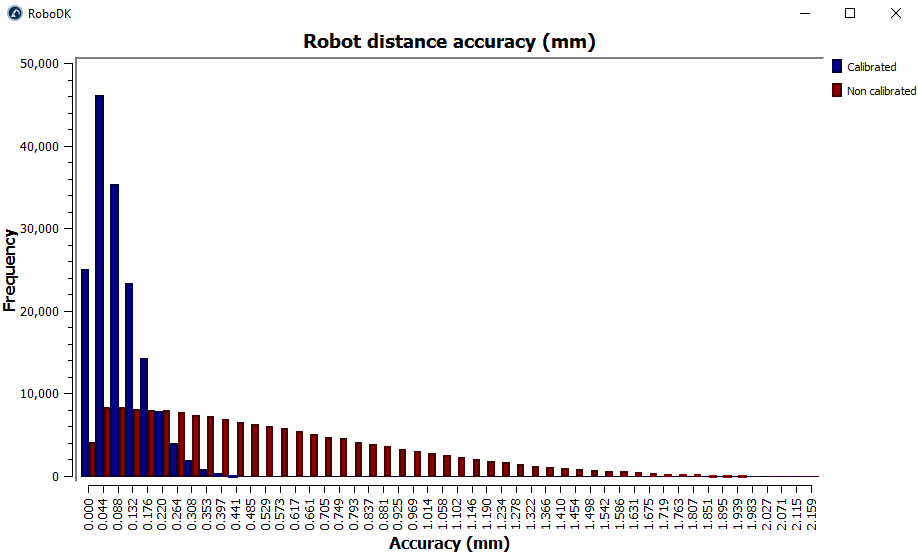
Select Show stats and two histograms will show the distribution of the errors before and after calibration, one histogram for position accuracy and the other showing distance accuracy. The following images correspond to the 315 validation measurements used in this example.
Finally, you can select Make report and a PDF report with the information presented in this section will be generated.
Program Filtering
Once the robot has been calibrated, you have different ways to use the robot calibration:
●Filter existing programs: all the robot targets inside a program are modified to improve the accuracy of the robot. It can be done manually or using the API.
●Use RoboDK for Offline Programming to generate accurate programs (generated programs are already filtered, including programs generated using the API).
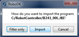
To filter an existing program manually: drag & drop the robot program file into RoboDK’s main screen (or select File➔Open) and select Filter only. The program will be filtered and saved in the same folder. The filter summary will mention if there were any problems using the filtering algorithm. You also have the option to import a program if you want to simulate it inside RoboDK. If the program has any dependencies (tool frame or base frame definitions, subprograms, ...) they must be located in the same directory where the first program is imported.


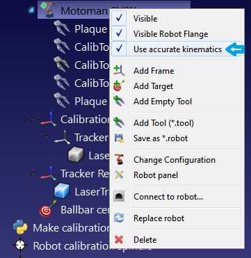
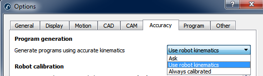
Once you import the program inside RoboDK you can regenerate it with or without absolute accuracy. In the main accuracy settings of RoboDK (Tools➔Options➔Accuracy) you can decide if you want to always generate the programs using accurate kinematics, if you want RoboDK to ask every time or if you want to use the current robot kinematics. The current robot kinematics can be changed by right clicking the robot and activating/deactivating the “Use accurate kinematics” tag. If it is active you’ll see a green dot, if it is not active, you’ll see a red dot.
Filter Programs using the API
It is possible to filter a complete program using RoboDK given a calibrated robot and the robot program using the FilterProgram call:
robot.FilterProgram(file_program)
A macro example called FilterProgram is available in the Macros section of the library. The following code is an example Python script that uses the RoboDK API to filter a program.
from robolink import * # API to communicate with RoboDK
from robodk import * # basic matrix operations
import os # Path operations
# Get the current working directory
CWD = os.path.dirname(os.path.realpath(__file__))
# Start RoboDK if it is not running and link to the API
RDK = Robolink()
# optional: provide the following arguments to run behind the scenes
#RDK = Robolink(args='/NOSPLASH /NOSHOW /HIDDEN')
# Get the calibrated station (.rdk file) or robot file (.robot):
# Tip: after calibration, right click a robot and select "Save as .robot"
calibration_file = CWD + '/KUKA-KR6.rdk'
# Get the program file:
file_program = CWD + '/Prog1.src'
# Load the RDK file or the robot file:
calib_item = RDK.AddFile(calibration_file)
if not calib_item.Valid():
raise Exception("Something went wrong loading " + calibration_file)
# Retrieve the robot (no popup if there is only one robot):
robot = RDK.ItemUserPick('Select a robot to filter', ITEM_TYPE_ROBOT)
if not robot.Valid():
raise Exception("Robot not selected or not available")
# Activate accuracy
robot.setAccuracyActive(1)
# Filter program: this will automatically save a program copy
# with a renamed file depending on the robot brand
status, summary = robot.FilterProgram(file_program)
if status == 0:
print("Program filtering succeeded")
print(summary)
calib_item.Delete()
RDK.CloseRoboDK()
else:
print("Program filtering failed! Error code: %i" % status)
print(summary)
RDK.ShowRoboDK()
Filter Targets using the API
The following code is an example Python script that uses the RoboDK API to filter a target (pose target or joint target), using the FilterTarget command:
pose_filt, joints = robot.FilterTarget(nominal_pose, estimated_joints)
This example is useful if a 3rd party application (other than RoboDK) generates the robot program using pose targets.
from robolink import * # API to communicate with RoboDK
from robodk import * # basic matrix operations
def XYZWPR_2_Pose(xyzwpr):
return KUKA_2_Pose(xyzwpr) # Convert X,Y,Z,A,B,C to a pose
def Pose_2_XYZWPR(pose):
return Pose_2_KUKA(pose) # Convert a pose to X,Y,Z,A,B,C
# Start the RoboDK API and retrieve the robot:
RDK = Robolink()
robot = RDK.Item('', ITEM_TYPE_ROBOT)
if not robot.Valid():
raise Exception("Robot not available")
pose_tcp = XYZWPR_2_Pose([0, 0, 200, 0, 0, 0]) # Define the TCP
pose_ref = XYZWPR_2_Pose([400, 0, 0, 0, 0, 0]) # Define the Ref Frame
# Update the robot TCP and reference frame
robot.setTool(pose_tcp)
robot.setFrame(pose_ref)
# Very important for SolveFK and SolveIK (Forward/Inverse kinematics)
robot.setAccuracyActive(False) # Accuracy can be ON or OFF
# Define a nominal target in the joint space:
joints = [0, 0, 90, 0, 90, 0]
# Calculate the nominal robot position for the joint target:
pose_rob = robot.SolveFK(joints) # robot flange wrt the robot base
# Calculate pose_target: the TCP with respect to the reference frame
pose_target = invH(pose_ref)*pose_rob*pose_tcp
print('Target not filtered:')
print(Pose_2_XYZWPR(pose_target))
joints_approx = joints # joints_approx must be within 20 deg
pose_target_filt, real_joints = robot.FilterTarget(pose_target, joints)
print('Target filtered:')
print(real_joints.tolist())
print(Pose_2_XYZWPR(pose_target_filt))
Robot Mastering
Once the robot has been calibrated, you usually need RoboDK to filter programs, therefore, a RoboDK license is required (a basic OLP license is enough for generating accurate robot programs once the robot has been calibrated). Filtering a program means that the targets in a program are altered/optimized to improve the accuracy of the robot, taking into account all the calibration parameters (about 30 parameters).
Alternatively, you can calibrate only the joint offsets plus the base and tool reference frames (4 joint offset parameters plus 6 parameters for the base frame plus 6 parameters for the tool frame). The calibration will not be as accurate as if you used the default complete calibration but it might allow entering certain parameters in the robot controller and not depend on RoboDK to generate robot programs.
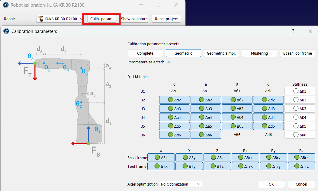
To obtain the calibration only for the joint offsets you must select the Calib. Param. button, then the Mastering button (inside the robot calibration menu).
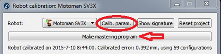

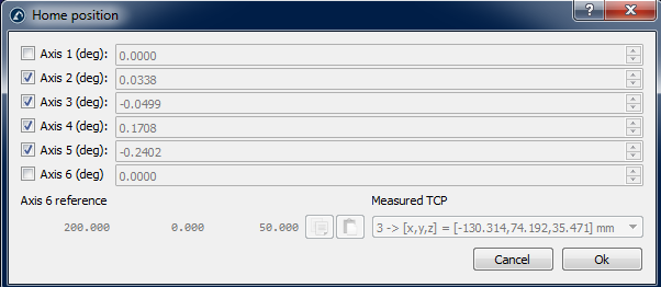
A new window will appear after you select Make mastering program. In this window you can select what axes you want to consider creating the new home position.
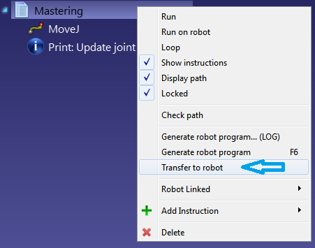
The button Make mastering program will appear in the robot calibration window. Select this button to generate a program that will bring the robot to the new home position. Transfer it to the robot and execute it, then, the new home position must be recorded.
If the robot and the PC are connected, you can right click the program and select Send Program to Robot to automatically send the program to the robot. Otherwise, you can select Generate robot program to see new joint values for the home position.
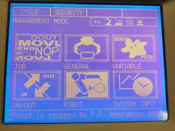
As an example, you must follow the next steps to update home position for Motoman robots.
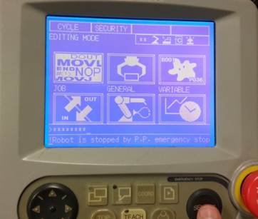
You must first run the program “MASTERING” to bring the robot to the new home position.
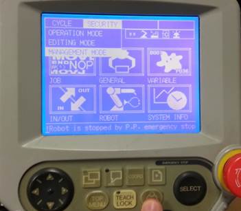
Once the program is in the controller you must log in as “Management mode” (password for Motoman robots is usually 99999999) and you need to be in Teach mode. The following images show the steps that must be followed.

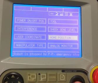
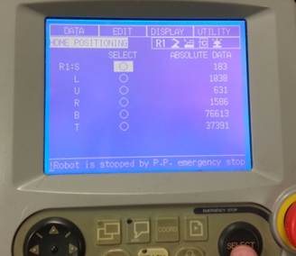
Make sure to update the home position for all robot joints.
Once the home position is set, you must delete the robot program that brought the robot to the new home position.
Reference frame and tool frame
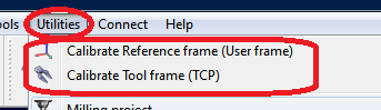
RoboDK provides some utilities to calibrate reference frames and tool frames. These tools can be accessed from Utilities➔Calibrate Reference frame and Utilities➔Calibrate Tool frame respectively.
To calibrate a reference frame or a tool frame (also known as User frame and TCP respectively) you need some robot configurations touching 3 or more points, these robot configurations can either be joint values or Cartesian coordinates (with orientation data in some cases). It is recommended to use the joint values instead of the Cartesian coordinates as it is easier to check the real robot configuration in RoboDK (by copy-pasting the robot joints to the RoboDK main screen).
Tool calibration
Select Utilities➔Calibrate tool to calibrate the TCP using RoboDK. You can use as many points as desired, using different orientations. More points and larger orientation changes are better as you will get a better estimate of the TCP as well as a good estimate of the TCP error.
The following two options are available to calibrate a TCP:
●By touching one stationary point with the TCP with different orientations.
●By touching a plane with the TCP (like a touch probe).
It is recommended to calibrate by touching a plane reference if we have to calibrate a touch probe or a spindle. This method is more stable against user errors.
If the TCP is spherical, the center of the sphere is calculated as the new TCP (it is not necessary to provide the sphere diameter).
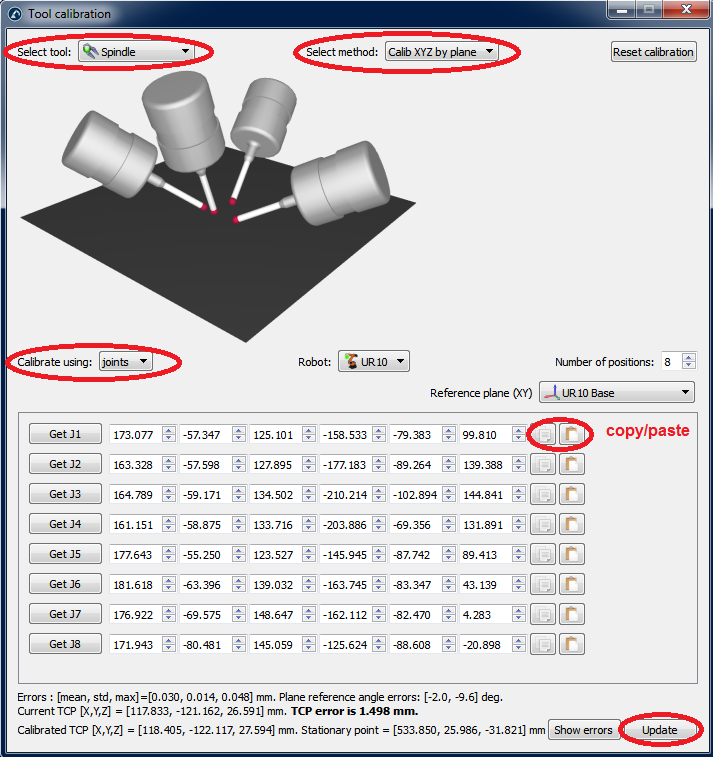
The following steps must be followed to calibrate the TCP with a plane (as seen in the picture):
1.Select the tool that needs to be calibrated.
2.Select the calibration method➔”Calib XYZ by plane”.
3.Select calibrate using “joints”.
4.Select the robot that is being used.
5.Select the number of configurations that you will use for TCP calibration (it is recommended to take 8 configurations or more).
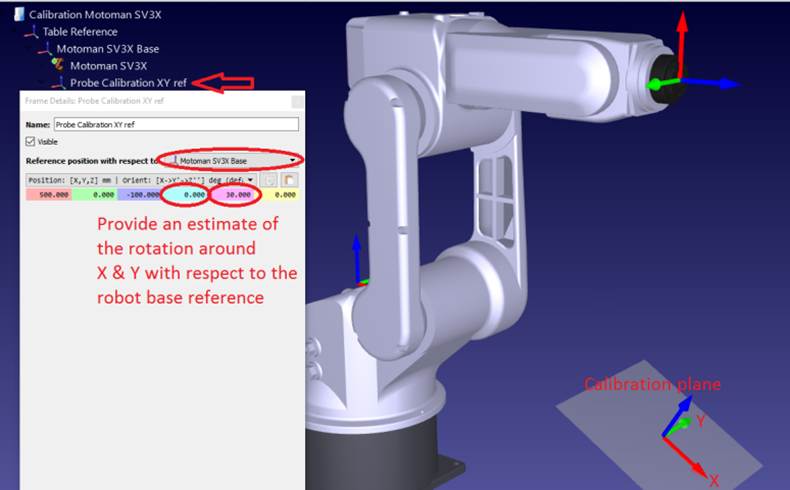
6.Select an estimate of the reference plane. If the reference plane is not parallel to the robot XY plane (from the robot reference) you must add an estimate of this reference plane within ±20 degrees. The position of this plane is not important, only the orientation.
7.You can start filling the table of joint values. You can fill it manually or by doing copy/paste with the buttons (as shown in the image). You can also use the button “Get Jx” to get the current joint values from the robot in the simulator. If you are getting the joints from a real robot connected to the robot you must first select “Get current joints” from the robot connection menu (see image attached or the appendix for more information about connecting a robot with RoboDK). It is strongly recommended to keep a separate copy of the joints used for calibration (such as a text file, for example).
8.Once the table is filled you will see the new TCP values (X,Y,Z) as the “Calibrated TCP”, towards the end of the window. You can select “Update” and the new TCP will be updated in the RoboDK station. The orientation of the probe cannot be found using this method.
9.You can select “Show errors” and you will see the error of every configuration with respect to the calculated TCP (which is the average of all the configurations). You can delete one configuration if it has a larger error than the others.
10.You must manually update the values in the real robot controller (X,Y,Z only). If this TCP will be used in a program generated by RoboDK, it is not necessary to update the values in the robot controller.
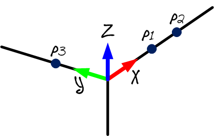
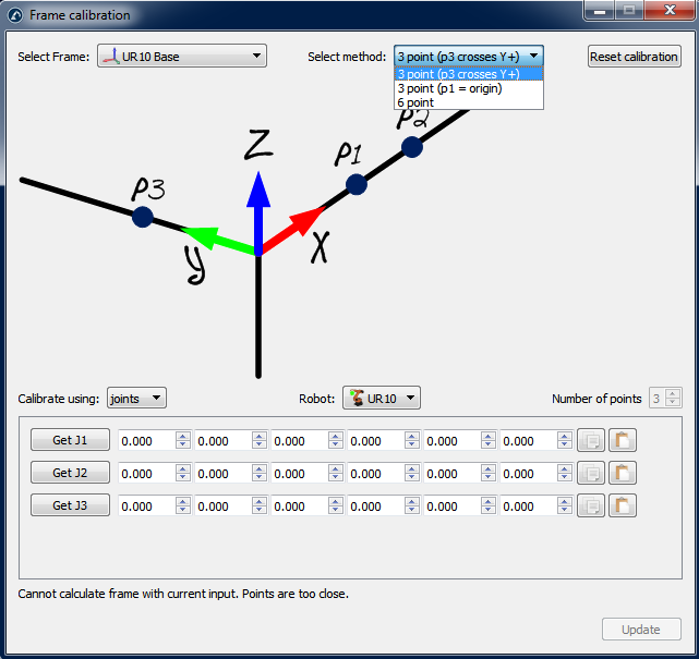
Reference frame calibration
Select Utilities➔Calibrate reference to calibrate a reference frame. It is possible to set a reference frame using different methods. In the example of the figure, a reference frame is defined by three points: point 1 and 2 define the X axis direction and point 3 defines the positive Y axis.
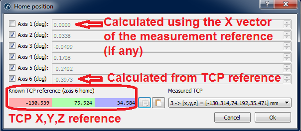
Annex I – Mastering for axes 1 and 6
You must pay special attention if you want to recover the mastering/home values for axes 1 and 6. These values are directly related to the robot base frame for the axis 1 and a TCP reference for axis 6. Therefore, external measurements must be taken to properly set these values. This window appears after you select “Make mastering program” in the calibration menu.
The next two procedures must be followed to properly set the mastering parameters for these two axes.
Axis 6 reference
You must use a reference target to properly set the “home” position of axis 6. The angle offset will be the rotation around the Z axis of the tool flange needed to best fit the measured TCP (X,Y,Z) with the known TCP reference. The measured TCP (see the following image) is one of the TCPs that were measured in the step two of the calibration procedure. The reference TCP is a known reference that corresponds to one of the TCP for the calibration tool being used.
Ideally, the reference TCP must be measured by the CMM with respect to the tool flange (a replica of the robot tool flange would be best). Alternatively, you can use a new robot to measure (step two of the calibration procedure) the TCP for the first time and use one measured TCP as the reference. It is important to use a dowel pin and/or appropriate tool flange referencing to make sure that the end effector is always placed at the same position.
Axis 1 reference
You must properly measure three base targets before starting a robot calibration if we want to align the axis 1 with the real robot base frame. These base targets must be chosen so that the reference frame can be found with respect to the robot.
The “home” position of axis 1 directly depends on the three base targets as well as the robot base setup. The robot base setup is the first calibration step, where the base frame of the measurement system is placed with respect to the robot base frame by moving and measuring axis 1 and 2.
The base targets of the measurement system can be set by pressing “Set base targets” (see following image). These are 3 measurements that will define the desired robot reference frame (the first 2 measurements define the X axis and the third point the positive Y axis). You should use appropriate reference points related to the robot base so that this procedure is repeatable.
The correction angle for joint 1 will be the angle between the X axis of the base reference measured through 3 points and the base reference measured by moving the robot axes 1 and 2. Of course, both vectors are previously projected to the XY plane of the base reference obtained by touching the tree points.

Annex II – Test the Faro laser tracker
Robot calibration requires measurements to be taken from the robot with a measurement system. To take these measurements it is required a Faro laser tracker that communicates with a computer. The communication is done through a driver exe file that can be run in console mode.
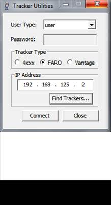
For example, Faro provides a free application called “Tracker Utilities”. This application can initialize the laser tracker and perform some health checks, among other things.
To initialize the tracker you should start the “Tracker Utilities” application, connect using the tracker IP, then, select “Startup Checks”. When the tracker initializes, you should place a 1.5’’ SMR target in the “home” position before initialization. Otherwise, the green light will flash after initialization and the measurements will not be valid.
Once the initialization is done you should read the “Startup complete” message, as shown in the following image.
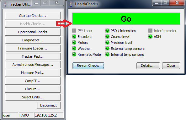
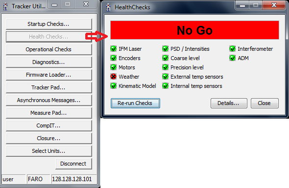
If you experience problems with the tracker, you can run some health checks by pressing “Health Checks…”. The next two images show a success check and a failed check respectively. Sometimes, problems are solved after reconnecting the cables and rebooting the laser tracker.

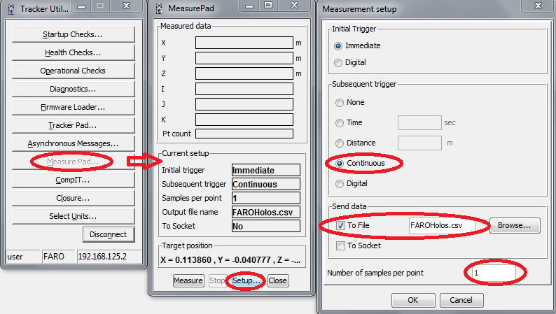
Finally, you can use the “Measure pad” to take some measurements. The laser tracker can follow a target and measure the XYZ position at a rate of 1000 Hz. If you set 1 sample per point and continuous trigger the tracker will record 1000 measurements per second in a CSV file.
You can use this feature to measure a robot path and use the RoboDK’s path accuracy check to check the accuracy, speed and acceleration along the path.